This Page Covers
ToggleHow to Use VLOOKUP in Excel - A Complete Beginner's Guide (With Examples)
Vlookup, people kept saying it was so important and it is complicated for beginners. But once understand how to use Vlookup Function. It can be use every single day at work, for pulling employee salaries, matching invoice numbers, or checking Product Prices
By the end of this post, you will know exactly what VLOOKUP does in a simplest way.
How to write it? , and How to fix it when it breaks?
What is VLOOKUP in Excel?
VLOOKUP stands for Vertical Lookup. It is a built-in Excel function that searches according to given criteria in a column and returns a value from another column in the same row.
Quite confusing right let me clear this to you, Imagine you have a data contains 100+ products names, bar codes along with their prices. You want to find the price of few product quickly without scrolling through all 100+ rows. VLOOKUP does that search for you instantly.
for example: You want to find 5 product’s prices and you just have barcodes of those 5 products so, you need to use vlookup function to pull prices of all 5 products instantly.
Understanding VLOOKUP Syntax
Before writing any formula, you need to understand its structure.
=VLOOKUP(lookup_value, table_array, col_index_num, [range_lookup])
There are 4 parts in Vlookup function each explained below
Lookup Value
The criteria searching for. It could be a product name, bar code, This is your search term.
For Example: selecting first barcode from the list of 5 barcodes.
Table Array
Selecting the range of data where Excel will do the search according to the given criteria / lookup value.
For Example: I have data of 100+ products in 3 columns, First Column have list of barcodes, Second have product names and Third have their prices. So, here I will select a range starting from first column to third column e.g. A2:C101.
Important Note: The first column of selected range must contain the criteria / lookup value you are searching for like the barcode which is in first column in my selected range of data
Column Index Number
Enter the column number from your selected range / table array that contains the result you want. Here we want to pull price which is on third of my selected range. So, here we need to type 3 as a column index number
Range Lookup
The TRUE or FALSE. enter 0 or FALSE for an exact match (commonly used & recommended). OR enter TRUE for an approximate match (rarely used).
Still have doubts? Don’t worry continue for step by step guide, today you will master VLOOKUP Function.
How to Use VLOOKUP in Excel? - Step by Step Guide
Lets go through with the real example, imagine you have the following data
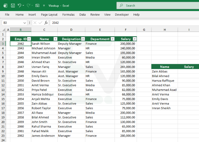
You want to find salaries of some employees listed on Column H (H9:H17)
Step 1 - Start writing VLOOKUP Formula
Click on the cell where you want the result to appear, for example H9 as here we are looking for Zain Abbas’ Salary first. Start typing in blank cell I9
=VLOOKUP(
Step 2 - Enter Lookup Value
Select lookup value, here the lookup value is Zain Abbas which is written in cell H9, Click on Cell H9 and type coma as shown below
=VLOOKUP(H9,
Step 3 - Select Table Array
Now Select a range of data where employee details are available.
Remember to start from the column where lookup value exist here the lookup value exist in Column C, so we need to select a range C3:F23 and type coma as shown below
=VLOOKUP(H9,C3:F23,
Step 4 - Enter the Column Index Number
Now give the column index number where result exist which is Column F 4th column of selected range C3:F23 like Column C is 1st (Name), D is 2nd (Designation), E is 3rd (Department), F is 4th (Salary) the result we are looking for, Now type 4 and coma as shown below
=VLOOKUP(H9,C3:F23,4,
Step 5 - Choose Exact Match
Now type FALSE or 0 and close bracket as show below
=VLOOKUP(H9,C3:F23,4,FALSE) or =VLOOKUP(H9,C3:F23,4,0)
Press Enter and see the result which is 125,000 the salary of Zain Abbas successfully rederived from selected range (Table Array)
This is the basic you just have learned this formula is good for now but as you know I have a list of many employee shown in H9:H17 and here we are looking for the salaries of all those employees.
If I drag the formula it will give some errors like #N/A and a hidden error.
Hidden Error of Vlookup
The hidden error Relative and Absolute Cell References
Learn Relative and Absolute Cell References.
Relative Cell Reference
It changes when copied or dragged relatively
View Example
=SUM(A4:C4) this formula is entered in Cell D4 when this cell is copied or dragged to D5 the formula will change relatively as =SUM(A5:C5)
Absolute Cell Reference
It will not change the range when copied or dragged
View Example
=SUM($A$4:$C$4) this formula has a range which remains the same where ever we copy or drag this formula because this range is locked using $ sign

See the example above when the first result in cell I9 is dragged or copied to I10:I17 the important selected range (Table Array) changed relatively which is the hidden error for some beginner users and caused incorrect results.
This range should be converted to Absolute Range by locking the selected range simply just by adding $ sign like: $C$3:$C$23
Shortcut: While selecting range (Table Array) just press F4 key to lock the range this will change your selected Relative range to Absolute Range as show below
C3:C23 with change into $C$3:$C$23